
A list of contracts is not a measure of diversification. What matters is how much independent movement survives after the contracts are put onto comparable risk and observed through time.
How much independent movement did six distinct futures markets actually provide?
Usually less than six—and materially less during periods of common stress.
Start with comparable daily movement
We selected one representative market from each of six economic groups: US 10-year Treasury futures, euro foreign exchange, the S&P 500, WTI crude oil, gold, and corn. The histories begin on 1 January 2000 and end on 27 August 2026.
Back-adjusted futures prices can cross zero or carry an arbitrary level after many contract rolls, so percentage returns are not always an appropriate input. Instead, each daily price change is divided by its own trailing 25-day standard deviation. This puts a large-dollar contract and a small-dollar contract on a comparable movement scale without pretending the adjusted price is an investable asset price.
Correlation is only half the picture
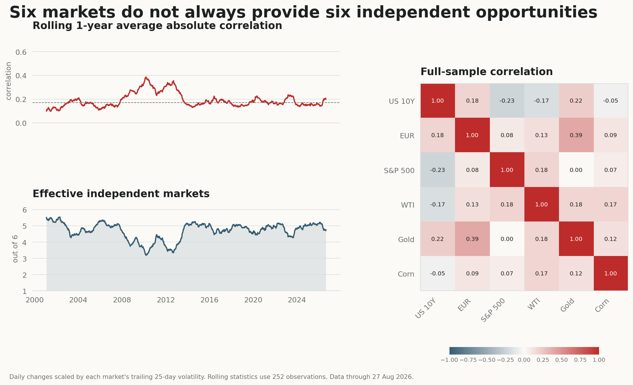
The upper panel averages the absolute value of all 15 pairwise correlations in each rolling year. Absolute correlation is deliberate: a persistent negative relationship can diversify a long-only collection, but it is still a strong common relationship that a directional system must understand.
The lower panel converts each six-by-six correlation matrix into an effective count. The calculation is the squared trace of the matrix divided by the sum of its squared eigenvalues. Six perfectly independent series score six. Six copies of the same series score one.
| Diagnostic | Observed value | Reading |
|---|---|---|
| Latest mean absolute correlation | 0.20 | Above the 0.17 sample median |
| Latest effective market count | 4.75 | Six contracts, about five independent dimensions |
| Lowest effective market count | 3.18 | Nearly half the apparent breadth disappeared |
The result is a warning against counting labels
Full-sample correlations look modest. The largest in the matrix is 0.39 between euro and gold; several pairs are close to zero. That is the reassuring view a single table provides. The rolling view is less comfortable. From the financial crisis into the European sovereign-debt period, common movement rose and the effective count fell toward three.
The portfolio problem is therefore dynamic. Asset-class labels help organise economic exposures, but they cannot certify independence. A useful hierarchy combines those labels with observed covariance, explicit group limits, and a willingness to reduce risk when yesterday's distinct markets begin behaving like one position.
Market count describes operational breadth. Effective market count describes statistical breadth. A robust portfolio needs to monitor both.
How this changed the engineering
Expanding a universe initially looks like a data-coverage task. In production it also creates an identity problem: instruments need stable metadata for asset class, sub-sector, geography, duration, and contract lineage. Without that structure, nearby equity indices or related rate contracts can quietly collect into a risk concentration while still appearing as separate rows.
The practical response is to make grouping part of the system rather than a presentation layer. Candidate markets are checked against both priced-volume measures and their correlation neighbours; portfolio reports use the same ignore lists and group definitions as the data and risk processes. That does not eliminate estimation error. It removes avoidable disagreement about what the portfolio owns.
Limits of this note
Six markets are an illustration, not the firm's trading universe. A 252-day window reacts slowly, while a shorter one would be noisier. Linear correlation misses tail dependence, liquidity shocks, and the asymmetry created by actual position signs. The chart also says nothing about forecast quality, costs, or expected return.
Its narrower conclusion is still useful: breadth is a quantity to estimate and stress, not a claim earned by adding another ticker.